5.2 Spatial Methods

spectral approach에서는 Laplacian eigenbasis을 이용하여 학습된 filter를 사용하게 되는데 이는 graph structure에 의존한다. 

spatial approach에서는 "define the convolution operation with differently sized neighborhoods and maintaining the local invariance of CNNs"

5.2.1 Neural FPS

[NIPS18] Convolutional networks on graphs for learning molecular fingerprints

• Key Idea: degree에 따라 다른 weight matrices을 사용$$x=h_{v}^{t-1} + \sum_{i=1}^{|N_v|} h_{i}^{t-1}$$ $$h_v^t = \sigma (x W_{t}^{|N_v|})$$
  • $W_t^{|N_v|}$: the weight matrix for nodes with degree $|N_v|$ at layer t
  • $N_v$: the set of neighbors of node v
  • $h_v^t$: the embedding of node v at layer t
• model first adds the embeddings from itself as well as its neighbors
• uses $W_t^{|N_v|}$ to do the transformation.
• the weight matrices with different node degrees
• Drawback: it cannot be applied to large-scale graphs with more node degrees

5.2.2 Patchy-SAN

• first selects and normalizes exactly k neighbors for each node.
• the normalized neighborhood serves as the receptive filed and the convolutional operation is applied.

1. Node Sequence Selection
2. Neighborhood Assembly
3. Graph Normalization
4. Convolutional Architecture

5.2.3 DCNN

  diffusion-convolutional neural networks

• "Transition matrices" are used to define the neighborhood for nodes in DCNN.

5.2.4 DGCN

 dual graph convolutional network

• consider the local consistency and global consistency on graphs.
• uses two convolutional networks to capture the local/global consistency and adopts and unsupervised loss to ensemble them.
•  
  • First Convolutional Network: uses the same equation as GCN
    • models the local consistency which indicates that nearby nodes may nhave similar labels.
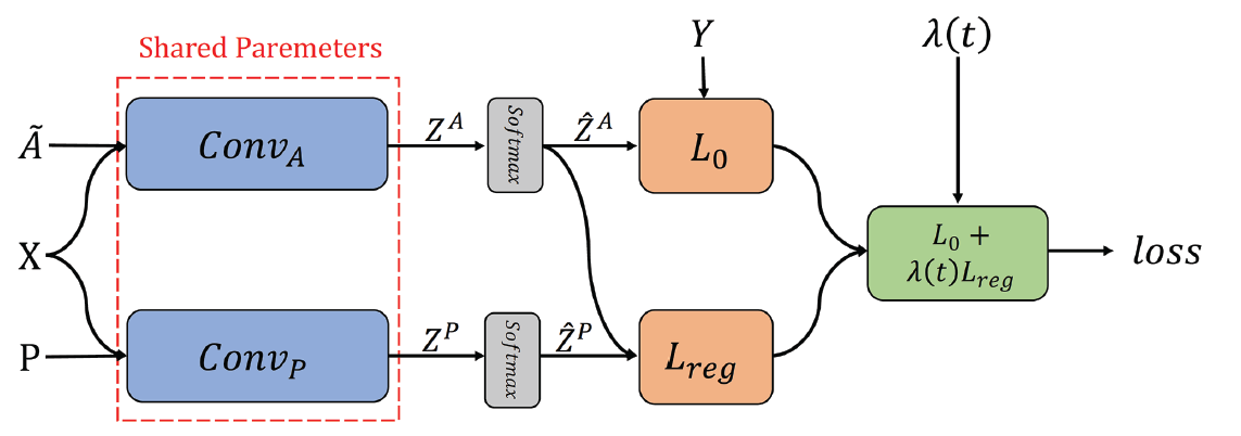
  • Second Convolutional Network: replaces the adjacency matrix with positive pointwise mutual information(PPMI) matrix $$H' = \sigma(D_{P}^{-\frac{1}{2}}X_P D_{P}^{-\frac{1}{2}}H\Theta)$$
    • $X_P$: the PPMI matrix
    • $D_P$: the diagonal degree matrix of $X_P$
    • $\sigma$: nonlinear activation function
    • models the global consistency which assumes that nodes with similar context may have similar labels.
  • Final Loss Function $$L=L_0 (Conv_A)+\lambda (t) L_{reg}(Conv_A, Conv_P )$$
    • $\lambda (t)$: the dynamic weight to balance the imporance of two loss functions
    • $L_0(Conv_A): supervised loss function with given node labels
    • $Z^A$: the output matrix of $Conv_A$
    • $\hat{Z}^A$: the output of $Z^A$ after a softmax operation
    • the loss $L_0(Conv_A)$: the cross-entropy error is as follows $$L_0(Conv_A)=-\frac{1}{|y_L|}\sum_{l\in   y_L} \sum_{i=1}^{c}Y_{l,i} ln(\hat{Z}_{l,i}^A)$$
      • $y_L$: the set of training data indices
      • $Y$: the ground truth
    • The calculation of $L_{reg}$ is calculated as follows: $$L_{reg}(Conv_A, Conv_P)=\frac{1}{n} \sum_{i=1}^{n} ||\hat{Z}_{i,:}^P - \hat{Z}{i,:}^A||^2 $$

Architecture of the dual graph convolutional network(DGCN) model

LGCN

Learnable Graph Convolutional Networks(LGCN)

• based on the learnable graph convolutional layer(LGCL) and the sub-graph training strategy.
• CNN을 aggregator로서 사용
• performs max pooling on nodes' neighborhood matrices to get top-k feature elements and then applies 1-D CNN to compute hidden representations $$\hat{H}_t = g(H_t, A, k)$$ $$H_{t+1} = c(\hat{H}_t)$$
  • $A$: the adjacency matrix
  • $g(\dot): the k-largest node selection operation
  • $c(\dot)$: the regular 1-D CNN
• model uses the k-largest node selection operation to gather information for each node.
• For a given node x, the features of its neighbors are firstly gathered
  • suppose it has n neighbors and each node has c features
  • a matrix $M\in \mathbb{R}^{n\times c}$ is obtained.(얻다)
  • $n < k$ 일 경우, 0으로 이루어진 column으로 M이 padding됨
  • Then the k-largest node selection is conducted that we rank the values in each column and select the top-k values.
  • After that, the embedding of the node $x$ is inserted into the first row of the matrix and finally get a matrix $\hat{M} \in \mathbb{R}^{(k+1)\times c}$
  • Then the model uses the regular 1-D CNN to aggregate the features
  • function $c(\dot)$ should take a matrix of $N\times (k+1)\times C$ as input and output a matrix of dimension $N\times D $ or $N\times 1 \times D$

An example of learnable graph convolutional layer(LGCL).

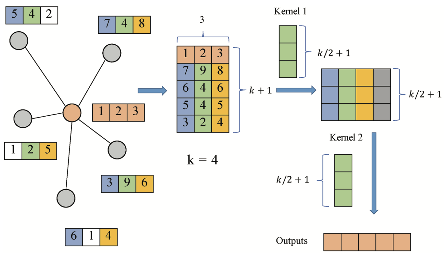
• Figure 예시
  • 각 노드는 3개의 feature로 이루어져 있음
  • 각 layer는 4개의 이웃들을 선택함, 즉 5개의 이웃들 중에서 4개를 select함
  • 두 개의 kernel을 이용하여 최종적으로 output길이가 5인 값이 출력됨

5.2.6 MoNet

non-Euclidean domain

• $x$: the node in the graph
• $y\in N_x$: the neighbor node of $x$
• u$(x,y)$: pseudo-coordinates between the node and its neighbor $$D_j(x)f = \sum_{y\in N_x}w_j(u(x, y))f(y)$$
  • $w_\Theta(u)=(w_1(u),../.w_J(u))$
• The spatial generalization of the convolution on non-Euclidean domain $$(f★g)(x)=\sum_{j=1}^{J} g_j D_j(x)f$$

5.2.7 GraphSAGE

a general inductive framework that generates embeddings by sampling and aggregating features from a node's local neighborhood

• The propagation step of GraphSAGE $$h_{N_v}^t = AGGREGATE_t (\{h_u^{t-1}, \forall u\in N_v\})$$
• AGGREGATE function
  • Mean aggregator
    • an approximation of the convolutional operation from the transductive GCn framework, so that the inductive version of the GCN variant could be derived by $$h_v^t = \sigma(W\dot MEAN(\{h_v^{t-1}\} \cup  \{h_u^{t-1} , \forall u \in N_v\})$$
    • mean aggreagator does not perform the concatenation operation which concatenates $h_v^{t-1}$ and $h_{N_v}^t$
    • can be viewed as a form of "skip connection"
  • LSTM aggregator
    • inputs in a sequential manner so that they are not permutation invariant
    • adat LSTMs to operate on an unordered set by permutating node's neighbors
  • Pooling aggregator
    • Each neighbor's hidden state is fed through a fully connected layer and then a max-pooling operation is applied to the set of the node's neighbors $$h_{N_v}^t = max(\{\sigma (W_{pool}h_u^{t-1} +b), \forall u \in N_u\})
• To learn better representations, GraphSAGE further proposes an unsupervised loss function which encourges nearby nodes to have similar representations while distant nodes have different representations $$J_G(z_u)=-log(\sigma(z_u^T z_v)) - Q \dot E_{v_n\sim P_n(v)}log(\sigma(-z_u^T z_{v_n}))$$