
- 분류 전체보기 (187)

- 주식경제 공부 (5)
- 머신러닝 (18)
- react 공부 (1)
- Docker 공부 (3)
- Kotlin실습 (3)
- 환경 설정 (6)
- linux, github, module 에러 정리 (15)
- python 간단 문법 정리 (12)
- pytorch module 정리 (5)
- github 관리하기 (7)
- protege (16)
- CS231N (2)
- goorm 수업 정리 (21)
- 취업일지 (8)
- 하둡 공부 정리 (0)
- paper study (8)
- algorithms (25)
- [CS224W] Machine Learning w.. (5)
- 화질 개선 프로젝트 (2)
- graph deep learning (15)
yuns
[KDD20] Policy-GNN: Aggregation Optimization for Graph Neural Networks 본문
[KDD20] Policy-GNN: Aggregation Optimization for Graph Neural Networks
yuuuun 2020. 12. 9. 03:50Abstract
GNN
- aim to model the local graph structures and capture the hierarchical patterns by aggregating the information from neighbors with stackable network modules.
- stack가능한 network module을 사용하여 neighbor들에 대한 정보를 aggregate함으로써 local graph structures을 모델링하고 hierarrchical pattern을 캡처하는 것을 목표로 함.
Introduction
Application
- anomaly detection
- molecular structure generation
- social network analysis
- recommendation system
One of the key techniques behind applications
- graph representation learning
- aims at extracting information underlying the graph-structured data into low dimensional vector representations.
- graph-structured data의 기본 정보를 저차원 벡터 표현으로 추출하는 것을 목표로 함.
A lot of momentum has been gained by graph convolution networks(GCNs) and graph neural Networks(GNNs)
2 directions of advancing GNNs
- sampling stategies
- ex) batch sampling and importance sampling
- proposed to improve learning efficiency.
- 단점) sampling strategy may cause information loss and thus delivers sub-optimal performance
Novel message passing Functions
- to better capture the information underlying the graph structures
- ex) pooling layers, multi-head attention
- focus on deep architectures and studied the oversmoothing problem, which leads to gradient vanishing and makes features of vertices to have the same value.
- skip-connection을 적용하는 것은 sub-optimal할 수 있음
- requires manually specifying the starting layer and the end layer for constructing the skip-connection.
advocate explicitly sampling diverse iterations of aggregation for different nodes to achieve the best of both worlds.
- 서로 다른 노드에 대해 다양한 집계 반복을 명시 적으로 샘플링하여 두 세계의 최고를 달성 할 것을 권장합니다.
이 논문에서는 구조적인 정보를 충분히 반영하기 위하여 노드들마다 다양한 aggregation의 반복을 요구한다고 가정한다. 하지만 실제 그래프는 일반적으로 여러 유형의 attribute들을 가지고 있어 복잡하고, 각 노드에 대한 적절한 aggregation strategy를 정의할 수 있긴 하나, 노드를 서로 다른 수의 network layer에 제공해야 되기 때문에 이러한 node에서 GNN을 훈련하는 것이 어렵다는 단점을 가지고 있다. 이에 Policy-GNN은 복잡한 aggregation strategy를 모델링하는 meta-policy framework를 제안한다. 이는 모델의 feedback를 활용하여 meta-policy를 최적화하는 Markov decision process(MDP)로서의 meta-policy를 적용한다.
Perliminaries
Problem Definition
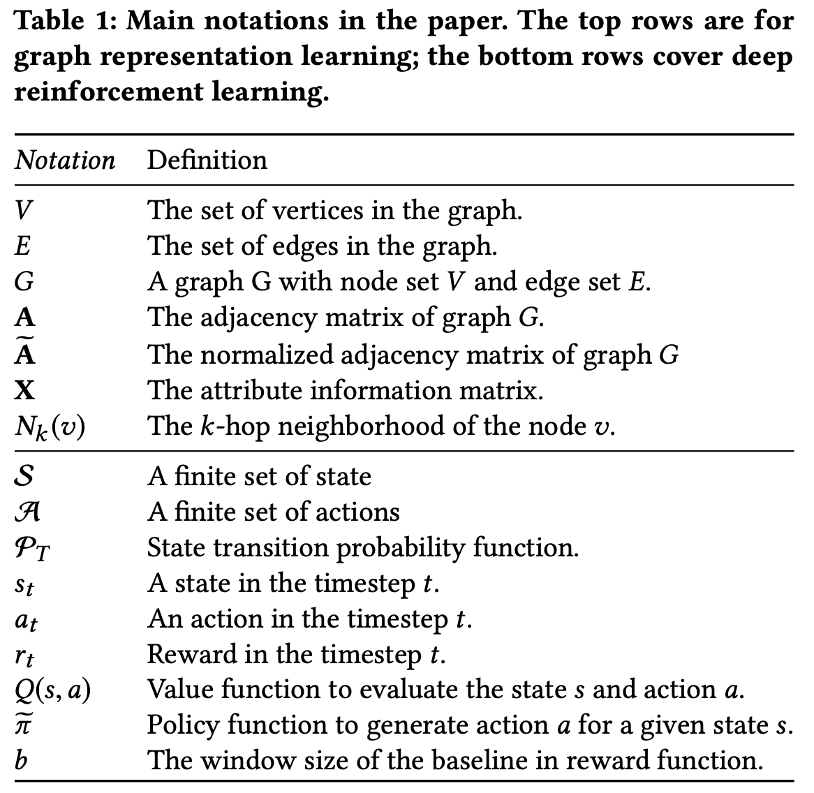
Symbols
- $G=(V,E)$ : a graph
- $V=\{v_1, v_2, v_3, \cdots, v_n\}$: the set of vertices
- $E\subseteq V\times V$: the set of edges
- $n$: the number of vertices in $G$
- Each edge $e=(u,v,w)\in E$
- $u\in V$: a start node
- $v\in V$: a end node
- $w\in \mathbb{R}^+$: edge weight (the strength of the relation between $u$ and $v$.
- $A\in \mathbb{R}^{n\times n}$: the convention of adjacency matrix
- $X\in \mathbb{R}^{n\times m}$: attribute information matrix to represent $G$
- $v'\in N_k(v)$: the k-order proximity of the node $v$.
- $N_k(v)$: for each node $v$, a set of k-hop neighborhoods
Graph representation learning
- aims embedding the graph into low-dimensional vector spaces(그래프를 저차원 벡터 공간에 삽입)
- goal: to learn the node representation through aggregating the information from $N_k(v)$
- the proximity information is preserved in the low dimensional feature vectors and the learned representations can be used in downstream tasks such as node clasification.
Problem of Aggregation Optimization
- Given an arbitrary graph neural network algorithm, the goal is to jointly learn a meta-policy $\tilde{\pi}$ with graph neural network
- $\tilde{\pi}$: maps each node $v\in V$ into the number of iterations of aggregation, such that the performance on downstream task is optimized.
Learning Graph Representations with Deep Neural Networks
Learning graph neural network consists of 3 steps
- intialization: intialize the feature vectors of each node by the attribute of the vertices
- neighborhood detection: determiner the local neighborhood for each node to further gather the information
- information aggregation: update the node feature vectors by aggregating and compressing feature vectors of the detected neighbors.
Methods of effectively gather the information from neighbors
- Graph Convolution Network(GCN)
- $\tilde{A}$: the normalized adjacency matrix where $\tilde{A}_{uv}=\frac{A_{uv}}{\sum_vA_{uv}}$
- feature. aggregation $$h_v^k = \sigma (\sum_{u\in\{v\}\cup N_1(v)} \tilde A_{uv}W_kh_u^{k-1})$$
- $W_k$: the trainable parameter in the k-th graph convolution layer
- $N_1(v)$: the one hop neighborhood of node $v$
- $h_u$ and $h_v$: $d$ dimensional feature vectors
- Graph Attention Network(GAT)
- to indicate the importance of the neighbors of a given node in aggregation
- $\tilde{A}$ : the self-attention scores, which indicate the importance of aggregation from node $u$ to node $v$.
- Improving the learning efficiency with sampling techniques
- two kinds of sampling strategy
- Local Sampling(proposed by GraphSAGE)
- performs aggregation for each node.(정해진 갯수만큼 sampling 진행)
- Global Sampling(proposed by FastGCN)
- introducing an imporance sampling among all of the nodes
- in order to build a new structure based on the topology of the original graph.
- Paper work
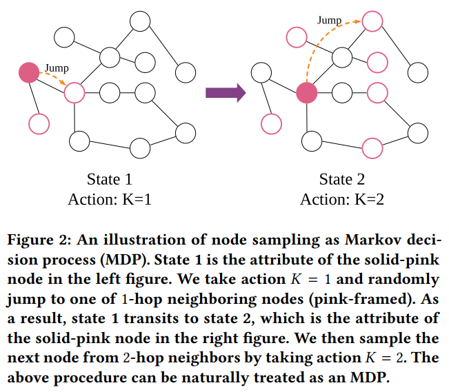
- formulate local sampling into Markov decision process
- learn the global infomation through training a meta-policy to make decisions on k-hop aggregation.
Sequential Decision Modeling with Markov Decision Process
Markov Decision Process(MDP)
- sequential decision making process
- 강화학습은 MDP의 문제를 푸는 것
- 의사 결정 과정을 모델링 하는 수학적 틀 제공
- MDP정리
- Symbol
- MDP $M$ is represented as quintuple $(S,A, P_T, R, \gamma)$
- $S$: a fomote set pf states
- $A$: a finite set of actions
- $P_T:S\times A\times S \rightarrow \mathbb{R}^+$: state transition probability function that maps the current state $s$
- $a$: action and the next state $s'$ to a probability
- $R:S \rightarrow \mathbb{R}$: the immediate reward function
- $\gamma \in (0, 1)$ discount factor
- At each timestep $t$, the agent takes action $a_t \in A$ based on the current state $s_t\in S$ and observes the next state $s_{t+1}$ as well as a reward state $r_t = R(s_{t+1})$.
- aim to search for the optimal decisions so as to maximize the expected discounted cumulative reward.
Solving Markov Decision Process with Deep Reinforcement Learning
- consider a model-free deep reinforcement learning, which learns to take the optimal actions through exploration.
- Deep-QLearning(DQN) uses deep neural networks to approximate state-action values $Q(s,a)$ that satisfies $$Q(s, a) = \mathbb{E}_{s'} [R(s') = \gamma \max_{a'}(Q(s', a'))]$$
- $s'$: the next state
- $a'$: the next action
- Two actions to stabilize the training
- a replay buffer to reuse past experiences
- a separate target network that is periodically updated.
Methodology
Meta-Policy module and a GNN module (Meta-Policy aims at learning the relations between node attributes and the iterations of aggregation)
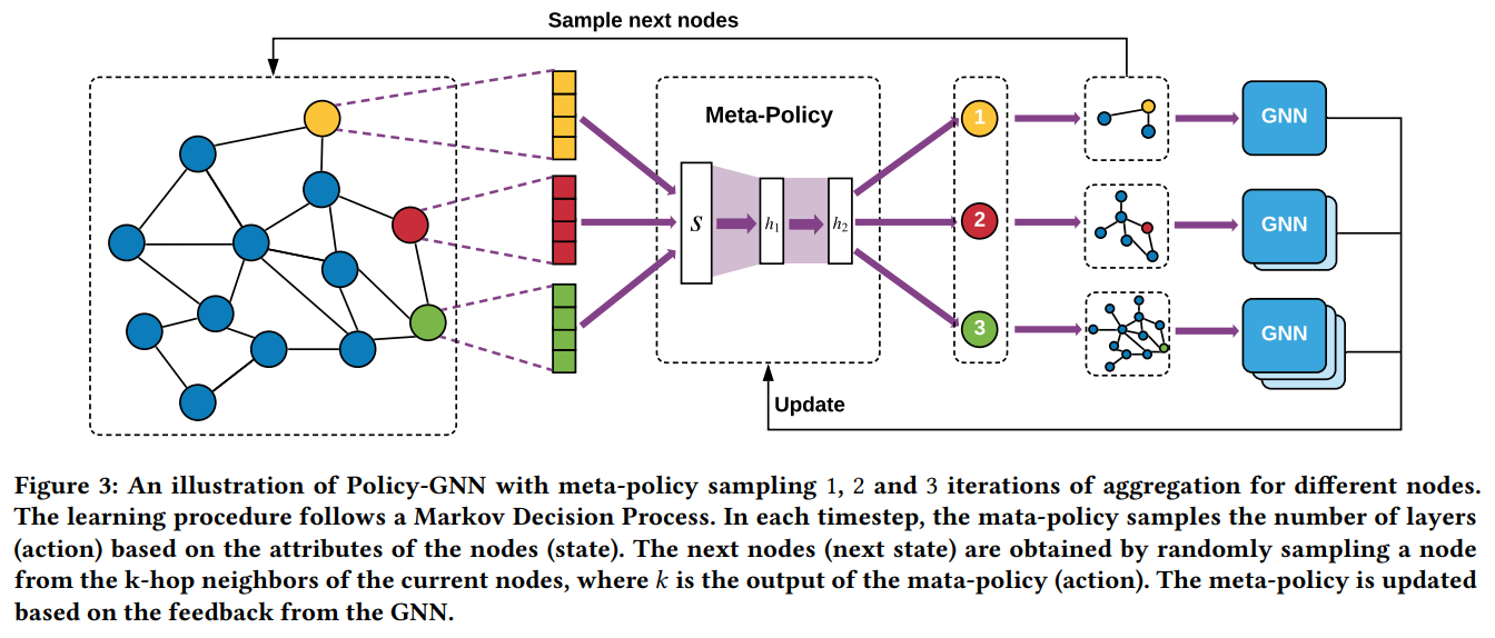
Step
- state: node attributes(the red/yellow/green feature vectors)
- maps the state into action(the number of hops shown in the red/yellow/green circles)
- sample the next state from the $k$-hop neighbors(the sub-graphs next to the action) of each node
- $k$: the output of the Meta-Policy(action)
- GNN module selects a pre-built $k$-layer GN architecture to learn the node representations and obtains a reward signal for updating the Meta-Policy.
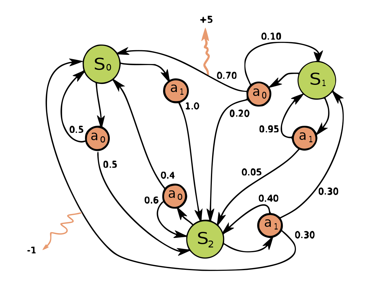
Aggregation Optimization with Deep Reinforcement Learning
- Discuss how the process of learning an optimal aggregation strategy can be naturally formulated as a Markov decision process(MDP).
- Key components
- states
- actions
- rewards
- transition probabilits - maps the current state and action into the next state.
- Definition
- State(S): The state $s_t \in S$ in timestep $t$ is defined as the attribute of the current node.
- Action(A): The action $a_t \in A$ in timestep $t$ specifies the number of hops of the current node.
- Reward Function(R): the reward $r_t$ in timestep $t$ as the performance improvement on the specific task comparing with the last state.
- Three phases
- selecting a start node and obtaining its attributes as the current state $s_t$
- generating an action $a_t$ from $\pi(s_t)$ to specify the number of hops for the current node
- sampling the next node from $a_t$-hop neighborhood and obtaining its attributes as the next state $s_{t+1}$.
- Proposition
- employ deep reinforcement learning algorithms to optimize the MDP.
- Since the action space of the aggregation process is a discrete space, deep Q-learning to optimize MDP
- i.e., $A \in \mathbb{N}$ and any arbitrary action $a \in A$ is always a finite positive integer
- Key factor in guiding the deep Q-learning is the reward signal
- a baseline in the Reward Function $$R(s_t, a_t) = \lambda(M(s_t, a_t) - \frac{\sum_{i=t-b}^{t-1}M(s_i, a_i)}{b-1}$$
- $\frac{\sum_{i=t-b}^{t-1}M(s_i, a_i}{b-1}$: the baseline for each timestep t
- $M$: the evaluation metric of a specific task
- $b$: a hyperparameter to define the window size for the historical performance to be referred for the baseline
- $\lambda$: a hyperparameter to decide the strength of reward signal
- $M(s_t, a_t)$: the performance of the task on the validation set at timestep $t$.
- a baseline function is to encourage the learning agent to achieve better performance compared with the most recent $b$ timesteps.
- a baseline in the Reward Function $$R(s_t, a_t) = \lambda(M(s_t, a_t) - \frac{\sum_{i=t-b}^{t-1}M(s_i, a_i)}{b-1}$$
- Reward함수를 이용하여 $Q(s, a) = \mathbb{E}_{s'} [R(s') = \gamma \max_{a'}(Q(s', a'))]$의 Q function을 학습시킨다. Epsilon-greegdy policy를 적용하여 policy function$\tilde{\pi}$ 획득
Graph Representation Learning with Meta-Policy
그래프에서 node representation할 때 aggregation하는 단계
The role that meta-policy plays in graph representation learning and how to learn the node embedding with Meta-Policy.
- Explicitly learn the aggregation strategy through the aforementioned meta-policy learning.
- Meta-Policy maps te node attributes to the number of hops --> action
- uses the number of number of hops to construct a specific GNN architecture for each node.
- Policy-GNN provides the flexibility to include all of the previous research fruits, including skip-connection, to facilitate graph representation learning.
Architecture consturction
- $$h_v^1 = \sigma (\sum_{u_1 \in \{ v \} \bigcup N_1(v)} \tilde{a}_{u_1v}W_1X_u)$$
- $$h_v^{k=a_t} = \sigma (\sum_{u_{k} \in \{ u_{k-1} \} \bigcup N_k(v)} \tilde{a}_{u_{k}u_{k-1}}W_1X_u^{k-1})$$
- $h_v^k$: the $d$ dimensional feature vector of node $v$ of the $k$ layer
- $X_u$: the input attribute vector of node $u$.
- $W_k$: trainable parameters of the $k$ laye
- $\sigma$: the ativation function of each layer
- $k=a_t$: the number of aggregation that decided by $\tilde{\pi}$ function in timestep $t$.
Accelerating Policy-GNN with Buffer Mechanism and Parameter Sharing
Re-constructing GNNs at every timestep is time-consuming, and the number of parameters may be large if we train multiple GNNs for different actions.
Parameter Sharing
- Reduce the number of training parameters via parameter sharing mechanism
- Initialize the maximum layer number $k$ of GNN layers in the beginning
- In each timestep $t$, repeatedly stack the layers by the initialization order for the action$a_t$ to perform GNN training.
- if number of hidden units for each layer is $n$: train $k\times n$ parameters rather than $\frac{nk(k+1)}{2}$
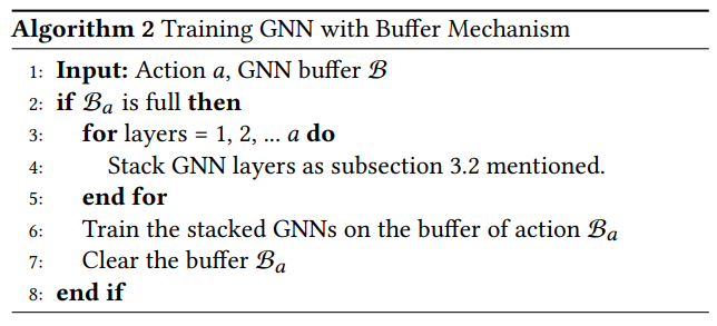
Buffer mechanism for graph representation learning
- After obtain a batch of nodes' attributes and a batch of actions, for each timestep, store them into the action buffer and check if the buffer has reached the batch size.
- If the buffer of a specific action is full, then construct the GNN with selected layers and train the GNN with the data in the buffer of the action.
- After the data has been trained on the GNN, clear the data in the buffer.
- If the batch size is too large, it will take much time, but still take less time than GNN.
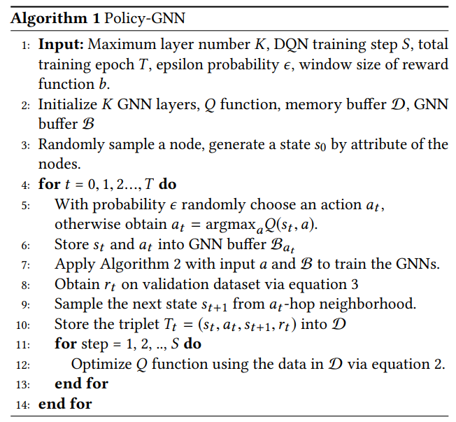
Detail of Algorithm
- Intialize $k$ GNN layer, $Q$ function, GNN buffer $B$, memory buffer $D$ for storation of the experiences.
- Randomly sample a batch of nodes and generate the first state with the node attributes
- Feed the state to $Q$ function and obtain the actions with $\epsilon$ probability to randomly choose the action
- Based on the chosen action, stack the layers from the initialized GNN layers in order
- Train the selected layers to get the feedback on the validation set.
- Obtain reward signal and store the transitions into a memory buffer -> randomly sample batches of data from the memory buffer and optimize the $Q$ function for the next iteration
Experiment
Focus
- How does Policy-GNN compare against the state-of-the-art graph representation learning algorithms?
- What does the distribution of the number of layers look like for a trained meta-policy?
- Is the search process of Policy-GNN efficient in terms of the number of iterations it needs to achieve good performance?
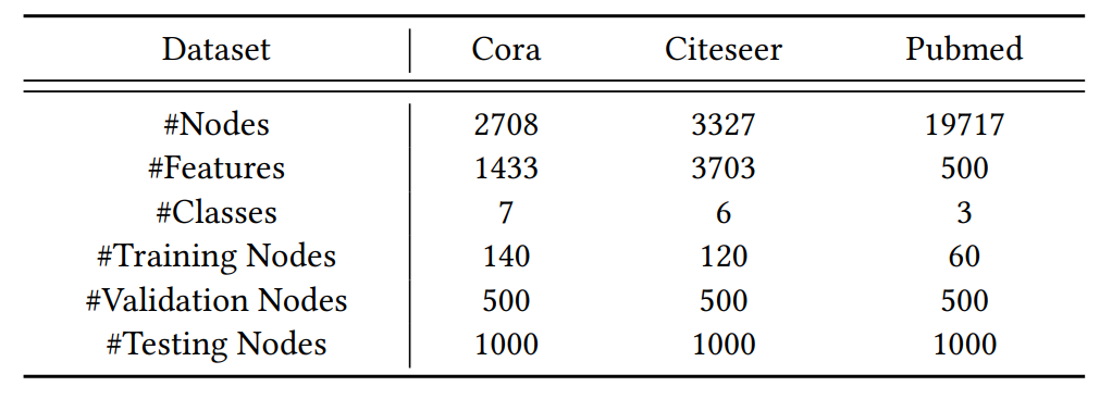
Datasets
Baselines
Three Categories
- Network Embedding
- skip-gram method
- DeepWalk
- Node2vec
- Static-GNNs
- Chebyshev
- GCN
- GraphSAGE
- FastGCN
- GAT
- LGCN
- Adapt
- g-U-Nets
- NAS-GNNs: neural atchitecture search based GNNs
- GraphNAS
- AGNN
'paper study' 카테고리의 다른 글
| ResNet (0) | 2020.12.09 |
|---|---|
| VGGNet (0) | 2020.12.09 |
| [KDD'19] KGAT: Knowledge Graph Attention Network for Recommendation (0) | 2020.01.16 |

